SML Lab VRP Solver

An educational tool for solving a class of VRPs incorporating single and multi depots, homogeneous and mixed fleets, delivery time windows, and open routes. Upload a spreadsheet, pick a solver, and compare heuristic vs exact solutions on an interactive map.

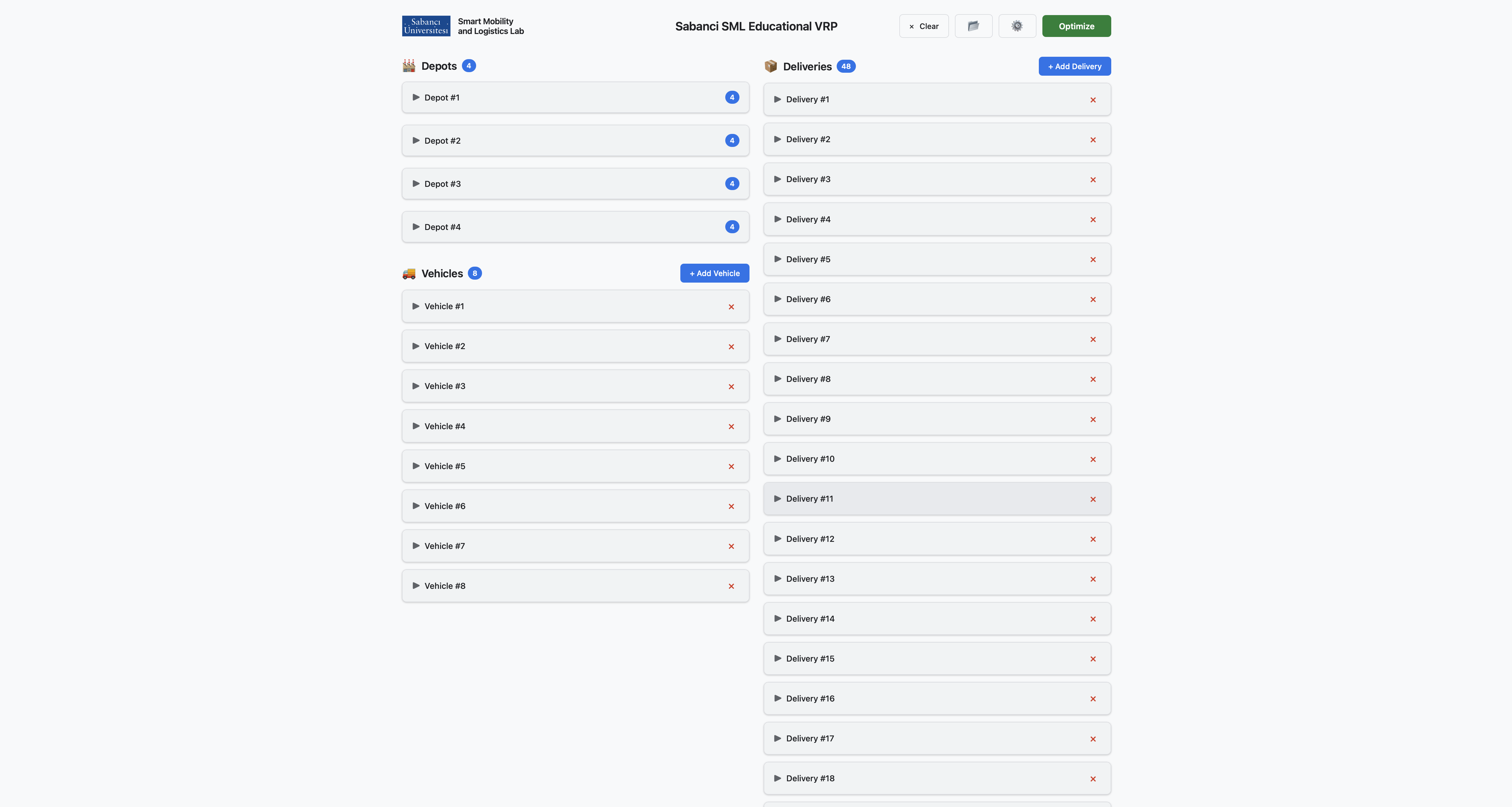
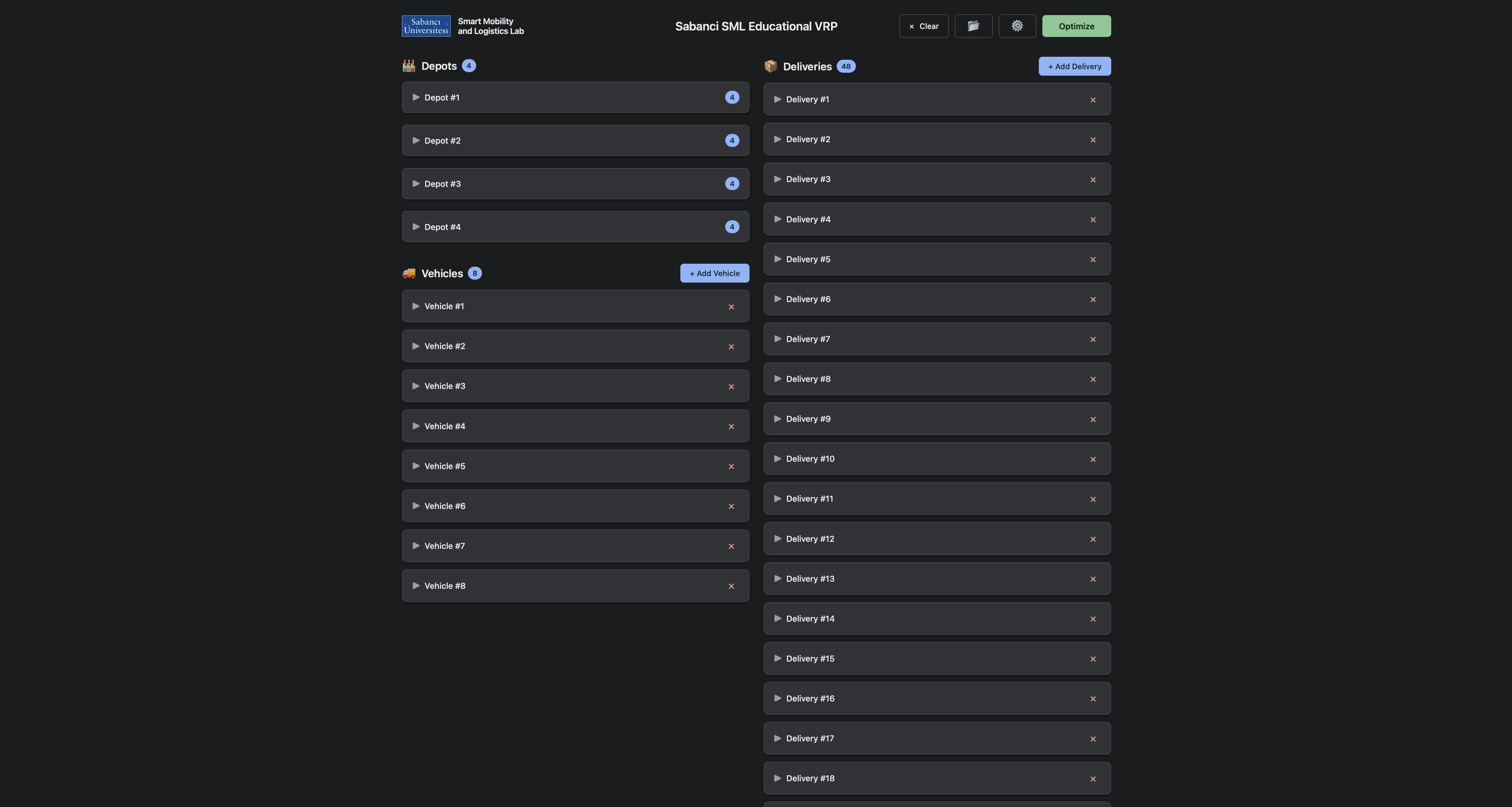
Open the optimizer Read the API docs

The optimizer input screen with vehicles and deliveries loaded

Built for classrooms, sized for experiments

Hard limits keep every run interactive, so a solver comparison fits inside a single lecture.

Deliveries per run: 50 max
Vehicles per run: 10 max
Neighbourhood operators: 14
Solve time limit: 600 s

One request body, two very different answers

Flip solverType between heuristic and exact and re-run the same instance. The comparison is the lesson.

Heuristic pipeline: Solomon I1 construction feeds an Adaptive Large Neighbourhood Search, which hands off to Variable Neighborhood Descent. Scales to the full 50-delivery limit and returns in seconds.
Exact MIP: An arc-based mixed-integer formulation solved with OR-Tools MathOpt on HiGHS. Proves optimality on small instances so students can see exactly how far a heuristic really is.
Same objective, same constraints: Both solvers minimize fixed plus travel cost under identical capacity, time-window, and route-duration constraints — so the numbers are directly comparable.
Same response shape: Identical OptimizationResponse either way: summary, per-vehicle routes with timed steps, encoded polyline geometry, and any unassigned deliveries.

Inside the heuristic

Three phases, fully inspectable

The heuristic solver is not a black box. The solver for the corresponding VRP variant combines three phases (construction, improvement, and refinement) that run in order, and each one is documented in the source.

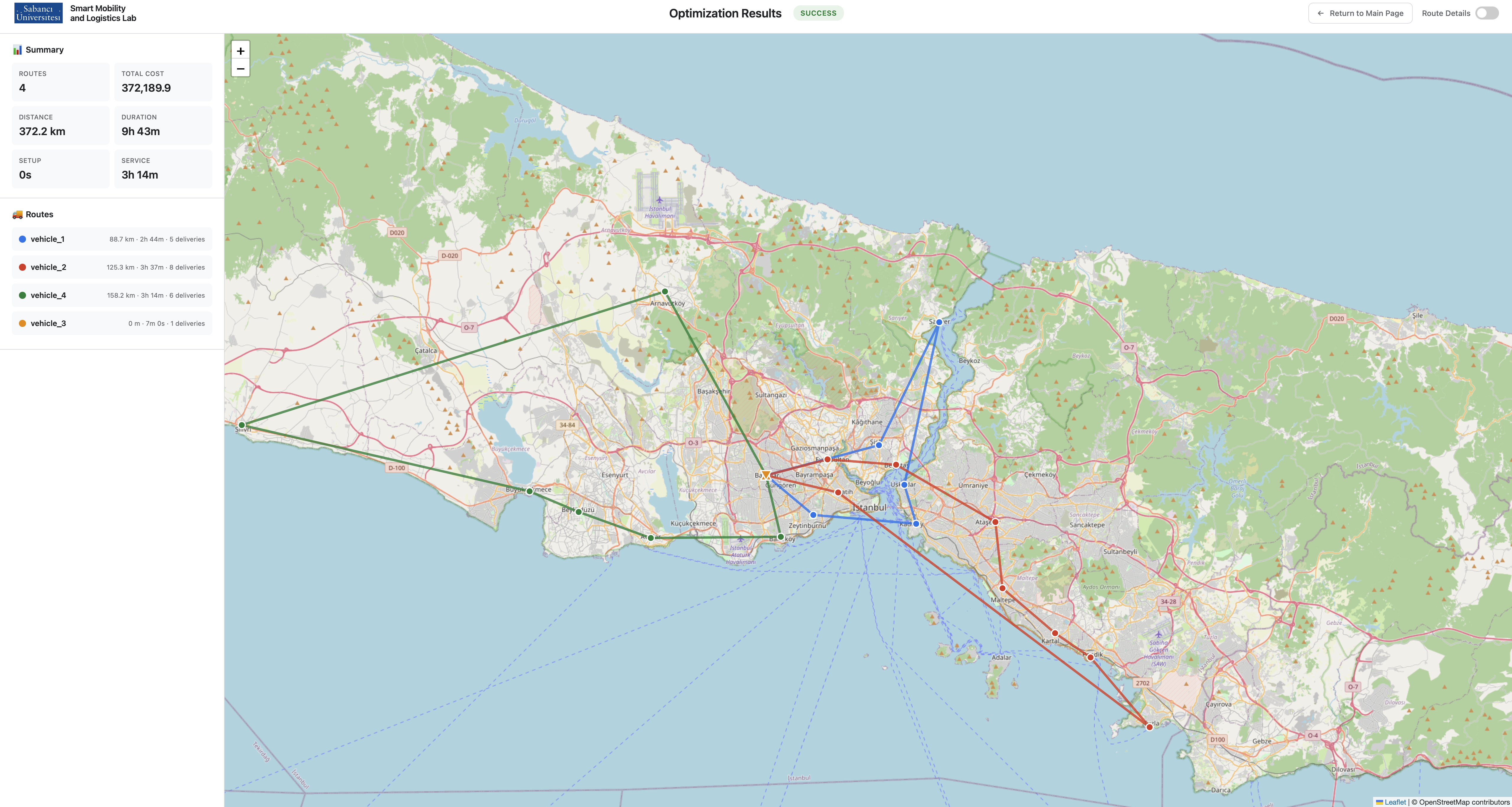
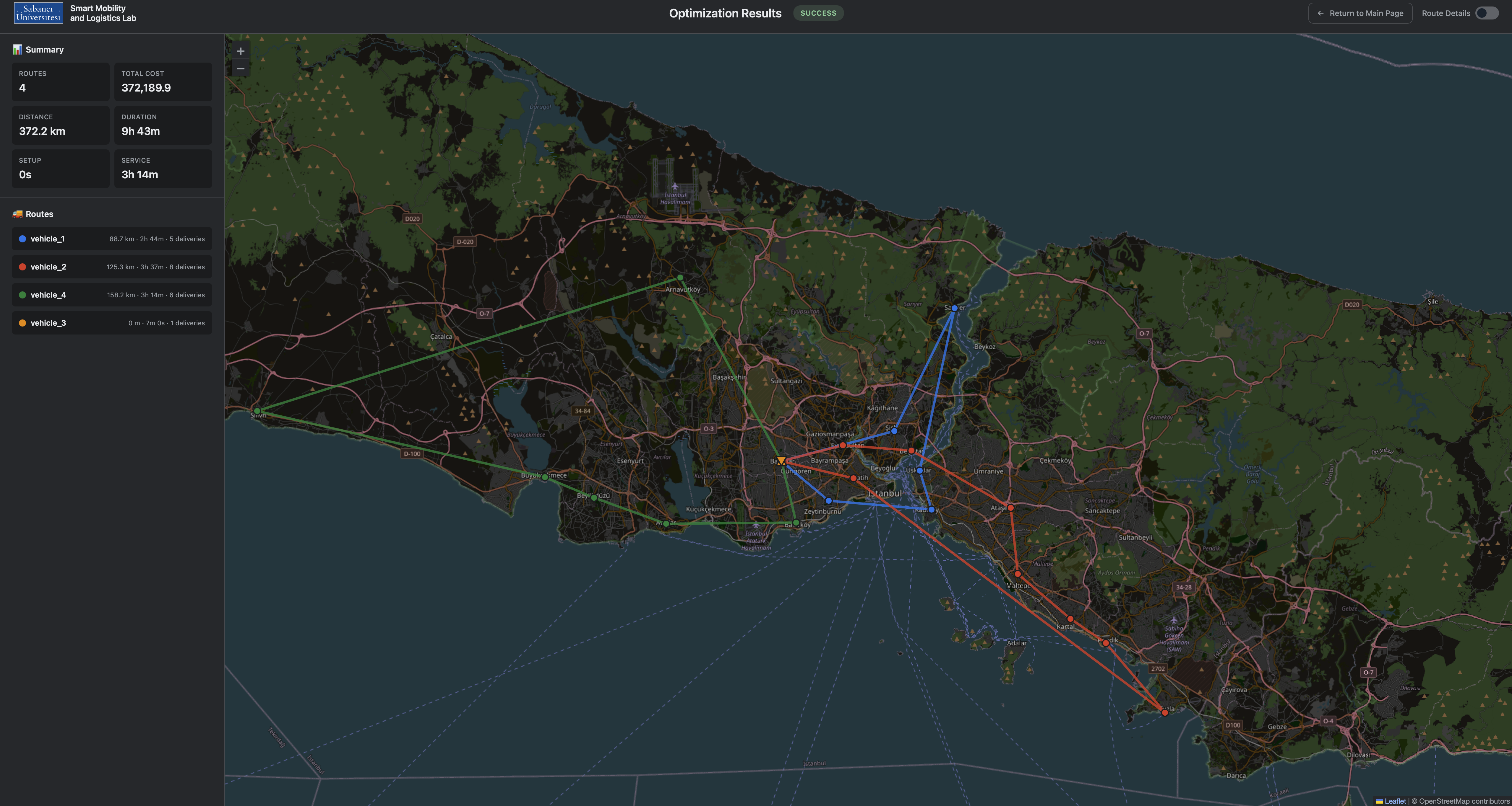
Optimized routes drawn on the results map

Each phase is a separate mixin with a single entry point, so you can run one, two, or all three and diff the results. The pipeline calls them in sequence: build a feasible solution, shake it hard and repair it thousands of times, then polish what is left.

Construction: Solomon I1. Vehicles open in fixed-cost order, then customers are inserted at the position that best balances travel-cost delta against time shift (α = 0.5, μ = 1.0), scored against a depot-distance benefit term (λ = 1.0).
Improvement: Adaptive Large Neighbourhood Search. Four destroy operators — random, worst, Shaw relatedness, and whole-route removal — pair with greedy and regret-2 insertion. A roulette wheel picks each pair, simulated annealing decides acceptance, and operator weights are rescored every 100-iteration segment.
Refinement: Variable Neighborhood Descent. Eight neighbourhoods run in a cycle that restarts on every improving move: or-opt and swap within routes, 2-opt, then relocate, or-opt, swap, 2-opt*, and cross-exchange across routes.

What you can model

A complete VRP lab, not just a solver

All VRP features are available on every request, including single/multiple depots, homogeneous/mixed fleets, delivery time windows, alternative return locations for routes, and a choice of distance model.

Real road networks.: Geographic mode pulls duration and distance matrices from the OSRM Table API and real driving geometry from the Route API.
Euclidean mode.: Swap in straight-line distances so textbook instances and synthetic benchmarks behave exactly as published.
Mixed fleet.: Per-vehicle capacity plus independent distance, time, and fixed cost coefficients — cheap vehicles open first.
Multiple depots.: Every vehicle has its own start and end location, and they do not have to match — model open routes or shift changes.
Time windows, loading and unloading.: Hard windows on every delivery and depot. Loading times are spent at the depot before the vehicle departs, and unloading times at each delivery stop.
Per-vehicle hard limits.: Cap maximum distance, maximum route time, and the number of deliveries any single vehicle is allowed to take.

REST API

Post an instance, get routes

A FastAPI service with automatic OpenAPI docs at /docs. Three endpoints are all you need.

POST /optimizer/solve.: Send deliveries, vehicles, mapType, solverType, and a timeout. Returns a status of success, partial, or infeasible with the full solution.
GET /optimizer/template.: Downloads the pre-formatted Excel workbook with Deliveries and Vehicles sheets.
POST /optimizer/upload-excel.: Upload a filled workbook and get back parsed deliveries and vehicles as JSON.

{
  "deliveries": [
    {
      "id": "delivery_1",
      "amount": 12,
      "start": {
        "latitude": 41.0082,
        "longitude": 28.9784,
        "timeWindow": [28800, 43200]
      },
      "end": {
        "latitude": 41.0082,
        "longitude": 28.9784
      },
      "setup": 60,
      "service": 300
    }
  ],
  "vehicles": [
    {
      "id": "vehicle_1",
      "capacity": 100,
      "start": {
        "latitude": 41.0255,
        "longitude": 28.9744
      },
      "end": {
        "latitude": 41.0255,
        "longitude": 28.9744
      },
      "cost": {
        "distance": 1,
        "time": 1,
        "fixed": 50
      },
      "constraints": {
        "maxTime": 28800,
        "maxDelivery": 20
      }
    }
  ],
  "mapType": "geographic",
  "solverType": "heuristic",
  "timeout": 60
}

{
  "status": "success",
  "summary": {
    "cost": 1842.6,
    "distance": 31204.0,
    "duration": 5460,
    "setup": 120,
    "service": 900,
    "routes": 2
  },
  "routes": [
    {
      "vehicle": "vehicle_1",
      "amount": 34,
      "cost": 921.3,
      "distance": 15602.0,
      "duration": 2730,
      "steps": [
        {
          "type": "start",
          "arrival": 28800,
          "load": 0
        },
        {
          "type": "delivery",
          "delivery": "delivery_1",
          "arrival": 29460,
          "distance": 4120.0,
          "load": 12
        },
        {
          "type": "end",
          "arrival": 31530,
          "load": 0
        }
      ],
      "geometry": "e{~vFvskeE…"
    }
  ],
  "unassigned": []
}

Getting started

Three ways in

Bring your own instance or start from one of the bundled datasets.

Start from the template

Download the Excel workbook, fill in the Deliveries and Vehicles sheets — amounts, coordinates, time windows, costs, and caps — then drag it into the app.

Download template

Load a sample dataset

Euclidean, Istanbul, and Türkiye instances are built in. Pick one from the upload dialog to see a solved run immediately.

Open the optimizer

Call the API directly

Post JSON to /optimizer/solve from a notebook or script. Interactive OpenAPI docs are generated automatically.

View API docs

Results

See the solution, not just the objective value

Routes render as real driving polylines on a Leaflet map, or as an SVG plot for Euclidean instances. Hover any stop for its arrival time, cumulative load, and distance travelled.

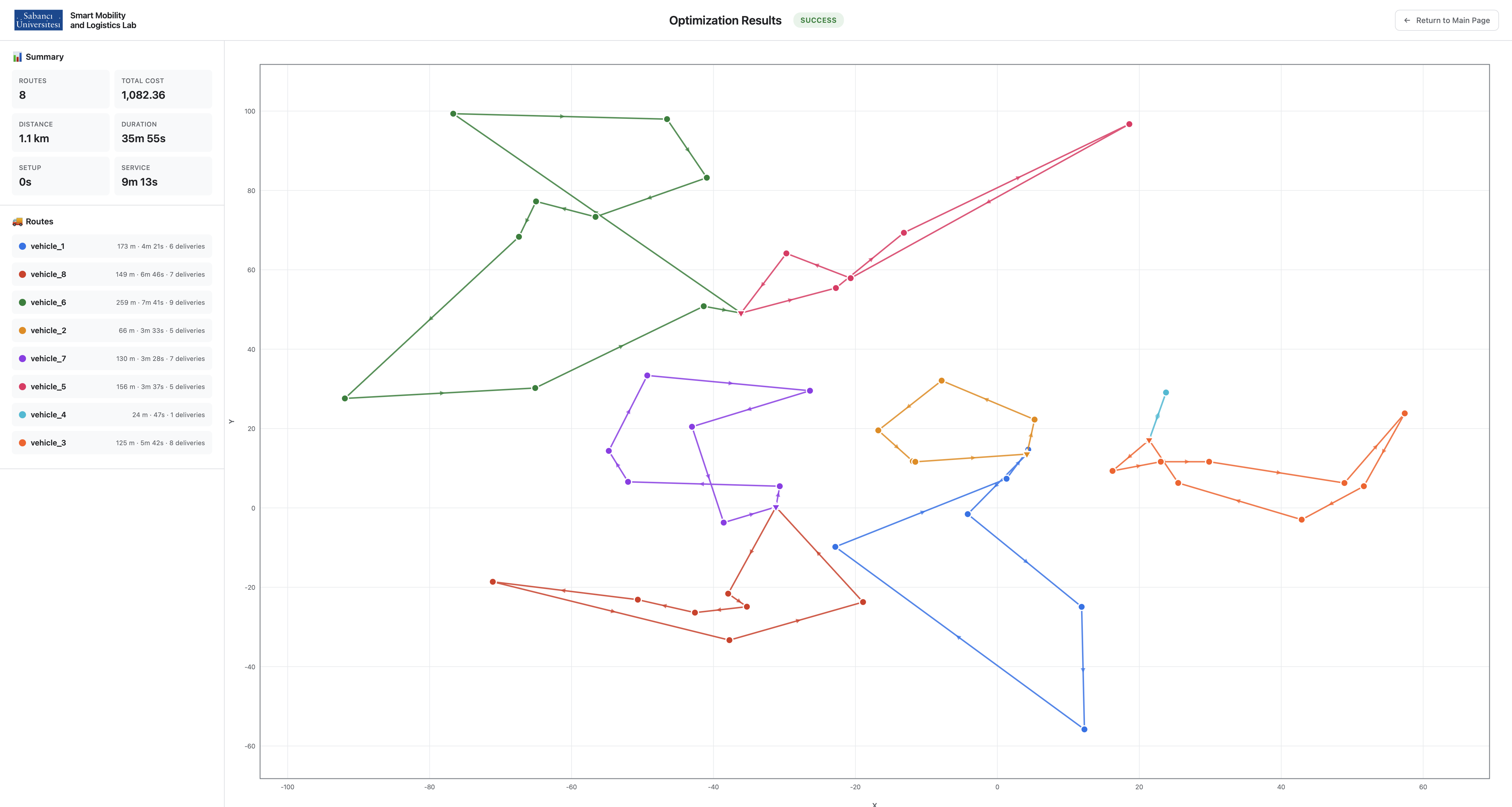
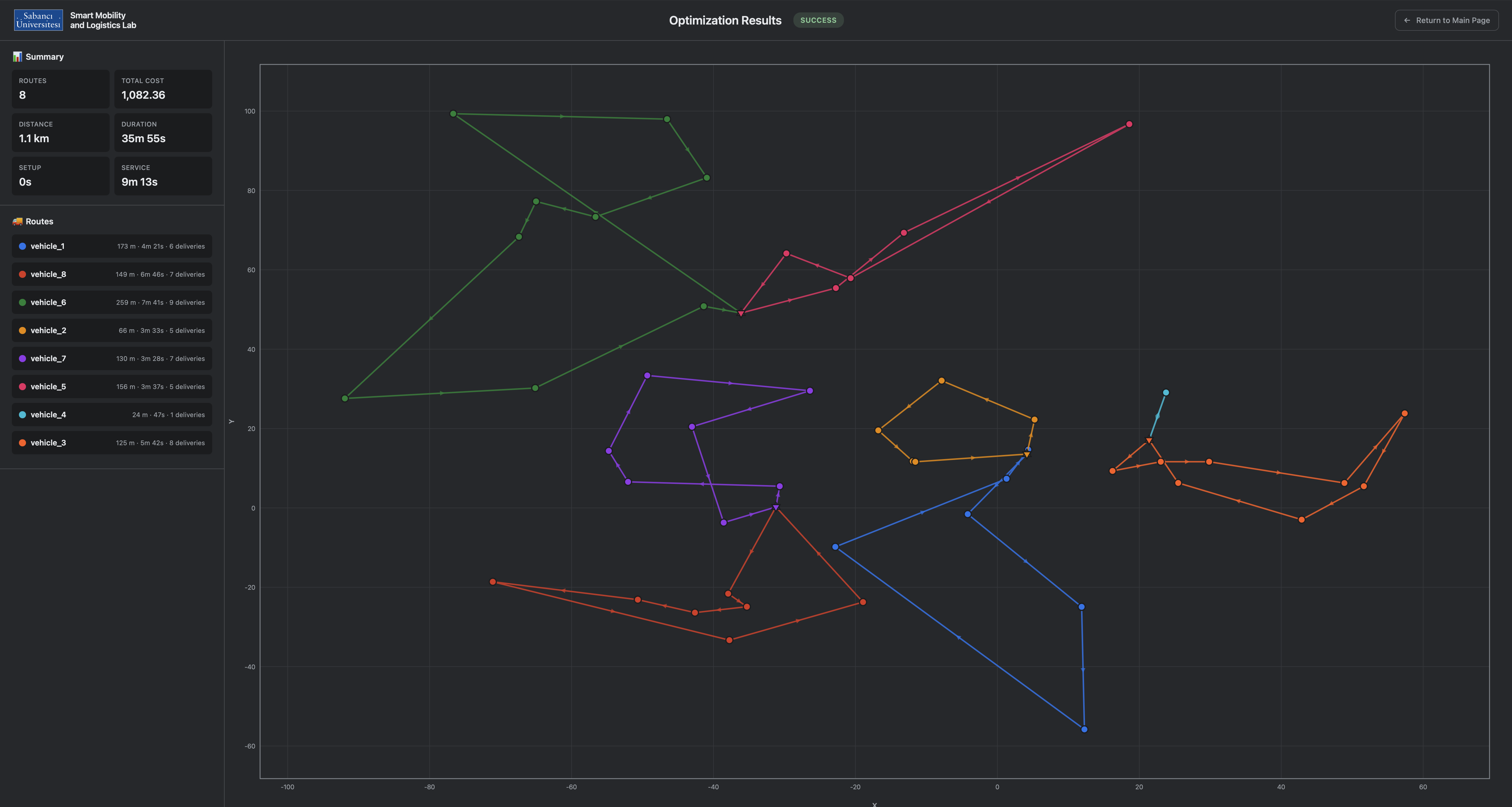
Results page showing a Euclidean instance plotted as an SVG scatter chart

Road-accurate polylines.: Geometry comes straight from the OSRM Route API, so a route follows actual streets rather than connecting dots.
Per-step timing.: Every stop reports arrival time, loading, unloading, and the distance covered to reach it.
Cumulative load.: Watch capacity fill and drain across a route to see exactly where a constraint binds.
Per-vehicle breakdown.: Cost, distance, duration, loading, and unloading totals for each route alongside the solution-wide summary.
Unassigned, made visible.: Deliveries no vehicle could serve are listed explicitly instead of disappearing from the map.
Euclidean plotting.: Textbook instances render as an SVG scatter plot with the same tooltips, no basemap required.

Frequently asked questions

: Single- and multi-depot problems with homogeneous or mixed fleets, delivery time windows, and open routes. In practice: vehicles may leave from and return to different locations, they do not have to share the same capacity or cost, and each delivery has to be served inside its time window. These features can be combined freely in the same instance.
: The heuristic pipeline for anything you would call an instance; the exact MIP for the handful of stops where you want a proven optimum to compare against. The MIP is an arc-based formulation with Big-M time propagation, so its size grows quickly — expect it to be useful up to roughly a dozen deliveries and to hit the time limit beyond that.
: In geographic mode, from an OSRM instance: one Table API call builds the duration and distance matrices, and one Route call per vehicle returns the polyline drawn on the map. In Euclidean mode, straight-line distance between coordinates is used for both, which is what published benchmark sets assume. You can point the service at your own OSRM server with the OSRM_URL environment variable.
: It comes back in an unassigned list and the response status becomes partial rather than success — nothing is silently dropped, and nothing is silently forced into an infeasible route. The results page shows unassigned deliveries in their own panel so you can see which constraint you over-tightened.
: The construction phase is deterministic. ALNS is not: it samples which deliveries to remove and accepts worse solutions probabilistically, and it also stops on a wall-clock budget, so two runs of the same instance can land on different solutions of similar cost. That variance is itself worth showing in a lecture — run the same instance twice and compare.
: Yes — it is a FastAPI service with a Dockerfile and a compose file. docker compose up serves it on port 8003; locally, uvicorn src:app is enough. Running it yourself also lets you raise the 50-delivery and 10-vehicle request caps and tune the ALNS and local-search parameters directly in src/core/constants.py.